Dragging Straight Lines in Python: Interactive Rate-Transient Analysis of a Tight-Oil Well
I have been working on unconventional wells recently and had to use an alternative to commercial software for the analysis when a licence was not available, or when the only available licence was being used by a colleague doing a similar task.
Rate-transient analysis (RTA) turns routine production data, rates and flowing pressures, into reservoir and fracture properties. For a multi-fractured horizontal well that means the permeability of the stimulated reservoir volume (kSRV), the effective fracture half-length, and the oil volume the fractures actually drain.
Most of the analysis is based on straight lines on specialised plots. In IHS Harmony, the tool used in the SPE paper below, you grab a line with the mouse, move it, and the results recalculate. OFM works in much the same way for decline-curve analysis (DCA).
The same type of analysis can be built in a plain Jupyter Notebook using Plotly and a few short Python functions.
The Paper
Li et al. (2018), SPE 189992, lays out a complete RTA workflow for a multi-fractured horizontal well in a tight-oil reservoir. Their Well 1 has 17 fracture stages along a 1,300 m lateral, 80 cp oil and about a year of daily data, the first 50 days of which are frac-fluid cleanup.
Figure 1: The RTA workflow of SPE 189992, simplified from the paper's Fig. 1. This note covers the three highlighted steps.
Data
The paper does not publish its production data, so synthetic data were generated for Well 1 from the information the paper does give: a closed-SRV linear-flow model with the Table 1 properties, and a bottomhole-pressure history shaped like the paper's Fig. 2. Cleanup, shut-ins, flush production after each shut-in, and measurement noise are all included.
The true values used to generate the data are:
- SRV permeability: 0.20 md, the value the paper's own Eq. 6 gives for its 156-day end of linear flow
- Fracture half-length: 39.2 m
- Oil in place in the SRV: 24.9×10⁴ m³
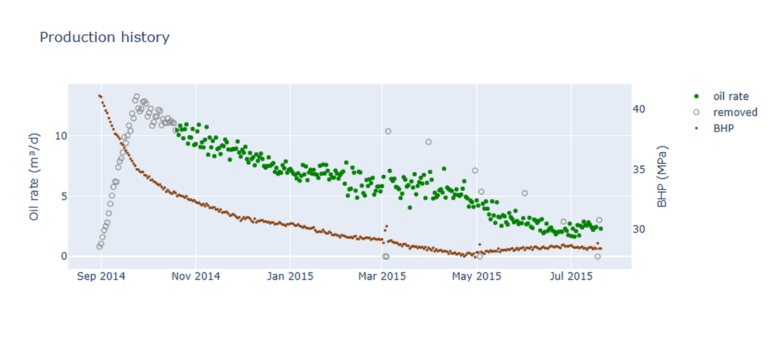
Figure 2: Synthetic Well 1, oil rate and bottomhole pressure. Hollow points are filtered out before the analysis (cleanup period, shut-ins, the day after each shut-in, and spikes), as in Fig. 2 of the paper.
Making a Chart Draggable
Plotly does most of the work. Its FigureWidget shows an interactive chart inside the notebook, and one setting lets the mouse move lines on it. What is left is telling Python what to do once a line has moved.
Here is the whole idea on the square-root-of-time chart:
sqrt_fig = go.FigureWidget()
sqrt_fig.add_scatter(x=sqrt_t, y=norm_pressure, mode='markers')  # the data
sqrt_fig.add_shape(type='line', x0=0, y0=0, x1=18, y1=3.5)  # the straight line
sqrt_fig._config = {'edits': {'shapePosition': True}}  # lets you drag it

def on_drag(layout, shapes):
    line = shapes[0]
    m = (line.y1 - line.y0) / (line.x1 - line.x0)  # slope of the line
    xf = eq5_xf(t_elf, m)  # paper Eq. 5
    sqrt_fig.layout.title = f'm = {m:.3f},  X_f = {xf:.1f} m'

sqrt_fig.layout.on_change(on_drag, 'shapes')
Every chart follows the same pattern: draw the data, add the line, and write one function that reads the line's new position and recalculates. The charts are linked the same way. Moving the end of linear flow on the diagnostic chart refits the lines on the √t and material-balance charts, as it does in commercial RTA software.
The same can be done in matplotlib with the ipympl backend and mouse events. Plotly needs less code, because dragging is built in. The results update when you let go of a line, not continuously while you drag.
Chart by Chart
The three charts below are live: drag the lines with the mouse, and the results in each chart title update when you let go. On this page the calculations run in JavaScript in your browser; the notebook runs the same equations in Python.
Flow-regime diagnosis (paper Fig. 4)
On log-log axes against material-balance time (cumulative production divided by rate), normalised rate shows two regimes. Transient linear flow into the fractures follows a half slope. Once the pressure disturbances from neighbouring fractures meet, boundary-dominated flow (BDF) follows a unit slope.
The key pick is the end of linear flow, Telf. As in the paper, this one line splits the two regimes: points before it are linear flow, and points after it are BDF, which feed the flowing material balance. The paper's Eq. 6 converts Telf directly into permeability:
where d is the fracture half-spacing, 38 m here. As in the paper, the constants are in field units.
Figure 3: Drag the green line, the end of linear flow. Points before it (blue) are linear flow, points after it (orange) are BDF. The blue and orange slope lines can be dragged too and keep their slopes.
One trap: the point where the half-slope and unit-slope lines cross is not Telf. It sits later, at roughly 2.5 times the dimensionless time that Eq. 6 assumes, so picking the crossing underestimates permeability by about that factor.
Square-root-of-time plot (paper Fig. 5)
In linear flow, normalised pressure Δp/q plotted against √t is a straight line. Its slope m gives the fracture half-length (Eq. 5):
The line refits automatically when Telf moves on the diagnostic chart. Both of its ends can also be dragged to place it by eye.
Figure 4: Drag either end of the red line to change its slope. A steeper slope means a shorter fracture. Moving the green line in Figure 3 refits it.
Flowing material balance (paper Fig. 7)
Once flow is boundary-dominated, normalised rate falls linearly with normalised cumulative production. Extending that line to zero rate gives the oil in place in the SRV. Since that volume equals 2·Xf·Le·h·φ·Soi (Eq. 8), it also gives a second estimate of fracture half-length.
Figure 5: Drag the end of the red line at zero rate to set the oil in place directly. Moving the green line in Figure 3 refits this line through the BDF points.
Results
With the end of linear flow picked at Telf = 163 days:
| Xf (m) | kSRV (md) | OOIPSRV (10⁴ m³) | |
|---|---|---|---|
| Telf + √t slope (paper Table 4 route) | 25.5 | 0.19 | 16.2 |
| Material balance + √t slope (paper Table 6 route) | 38.6 | 0.07 | 24.5 |
| Paper, Well 1 | 39.2 | 0.13 | 23.9 |
| Synthetic truth | 39.2 | 0.20 | 24.9 |
One observation worth mentioning: permeability depends on the pick. Eq. 6 recovers 0.19 md against a true 0.20 md, but only because Telf was picked well. Dragging it from 163 to 120 days raises permeability to 0.26 md.
What Interactivity Buys
The equations in this workflow take seconds, but the interpretation takes time: where linear flow ends, which points belong to BDF, and where the line really sits in noisy data.
A static script hides those decisions in parameters. A draggable chart puts them on screen, and every drag is a sensitivity case. Move Telf by six weeks, and permeability changes by more than a third.
That is why commercial RTA tools are built around interaction. In Python, it takes one short function per chart.
Takeaways
- The paper's straight-line workflow (diagnostic plot, √t plot, flowing material balance) runs in a Jupyter notebook with draggable lines, like IHS Harmony, or OFM for DCA.
- Plotly's
FigureWidgetdoes the dragging. Each chart needs one short Python function that recomputes when a line is moved. - It is a practical option when no commercial licence is available, or the licence is taken.
- Oil in place from flowing material balance is the most robust result: it is within 2% on the synthetic well.
- Permeability from Eq. 6 is only as good as the end-of-linear-flow pick, and dragging shows how sensitive it is.
- The √t slope assumes constant rate. For wells produced at near-constant pressure, it underestimates fracture half-length.
Code
The notebook and the synthetic dataset are on GitHub. Running it needs plotly and anywidget (pip install plotly anywidget). The charts are interactive in Jupyter and VS Code.
References
Li, H., Luo, H., Zhang, J. and Wang, J. (2018). Rate-Transient Analysis in Multifractured Horizontal Wells of Tight Oil Reservoir. SPE Production & Operations. SPE-189992-PA.
Wattenbarger, R.A., El-Banbi, A.H., Villegas, M.E. et al. (1998). Production Analysis of Linear Flow Into Fractured Tight Gas Wells. SPE-39931-MS.
Mattar, L. and Anderson, D. (2005). Dynamic Material Balance (Oil or Gas-In-Place Without Shut-Ins). PETSOC-2005-113.